stroup.splitplot {agridat}

Split-plot experiment of simulated data

Description

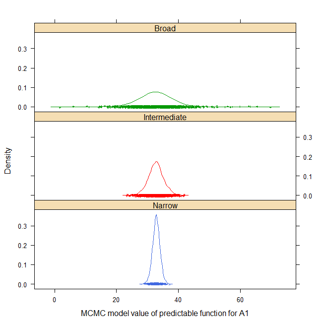
A simulated dataset of a very simple split-plot experiment, used to illustrate the details of calculating predictable functions (broad space, narrow space, etc.).

For example, the density of narrow, intermediate and broad-space predictable function for factor level A1 is shown below (html help only)

Format

y

simulated response

rep

replicate, 4 levels

b

sub-plot, 2 levels

a

whole-plot, 3 levels

Used with permission of Walt Stroup.

Source

Walter W. Stroup, 1989. Predictable functions and prediction space in the mixed model procedure. Applications of Mixed Models in Agriculture and Related Disciplines.

References

Wolfinger, R.D. and Kass, R.E., 2000. Nonconjugate Bayesian analysis of variance component models, Biometrics, 56, 768–774. https://doi.org/10.1111/j.0006-341X.2000.00768.x

Examples

## Not run: 
  
  library(agridat)
  data(stroup.splitplot)
  dat <- stroup.splitplot

  # ---- lme4 ---
  # libs(lme4)
  # m0 <- lmer(y~ -1 + a + b + a:b + (1|rep) + (1|a:rep), data=dat)
  # No predict function
  
  # ----- nlme ---
  # libs(nlme)
  # m0 <- lme(y ~ -1 + a + b + a:b, data=dat, random = ~ 1|rep/a)
  
  # ----- ASREML model ---
  if(require("asreml", quietly=TRUE)){
    libs(asreml,lucid)
    m1 <- asreml(y~ -1 + a + b + a:b, random=~ rep + a:rep, data=dat)
  
    # vc(m1) # Variance components match Stroup p. 41
    ##   effect component std.error z.ratio bound
    ##      rep    62.42     56.41      1.1     P
    ##    a:rep    15.39     11.8       1.3     P
    ## units(R)     9.364     4.415     2.1     P
    
    # Narrow space predictions
    predict(m1, data=dat, classify="a", average=list(rep=NULL))
    #  a Predicted Std Err    Status
    # a1     32.88   1.082 Estimable
    # a2     34.12   1.082 Estimable
    # a3     25.75   1.082 Estimable
    
    # Intermediate space predictions
    predict(m1, data=dat, classify="a", ignore="a:rep",
            average=list(rep=NULL))
    #  a Predicted Std Err    Status
    # a1     32.88    2.24 Estimable
    # a2     34.12    2.24 Estimable
    # a3     25.75    2.24 Estimable
    
    # Broad space predictions
    predict(m1, data=dat, classify="a")
    #  a Predicted Std Err    Status
    # a1     32.88    4.54 Estimable
    # a2     34.12    4.54 Estimable
    # a3     25.75    4.54 Estimable
  }    

  # ----- MCMCglmm model -----
  # Use the point estimates from REML with a prior distribution
  libs(lattice,MCMCglmm)
  prior2 = list(
    G = list(G1=list(V=62.40, nu=1),
             G2=list(V=15.38, nu=1)),
    R = list(V = 9.4, nu=1)
  )
  m2 <- MCMCglmm(y~ -1 + a + b + a:b,
                 random=~ rep + a:rep, data=dat,
                 pr=TRUE, # save random effects as columns of 'Sol'
                 nitt=23000, # double the default 13000
                 prior=prior2, verbose=FALSE)

  # posterior.mode(m2$VCV)
  #       rep     a:rep     units 
  # 39.766020  9.617522  7.409334
  # plot(m2$VCV)

  # Now create a matrix of coefficients for the prediction.
  # Each column is for a different prediction.  For example,
  # the values in the column called 'a1a2n' are multiplied times
  # the model coefficients (identified at the right side) to create
  # the linear contrast for the the narrow-space predictions
  # (also called adjusted mean) for the a1:a2 interaction.
  #              a1n   a1i  a1b a1a2n a1a2ib
  cm <- matrix(c(1,   1,   1,    1,    1,   # a1
                 0,   0,   0,   -1,   -1,   # a2
                 0,   0,   0,    0,    0,   # a3
                 1/2, 1/2, 1/2,    0,    0,   # b2
                 0,   0,   0,  -1/2,  -1/2, # a2:b2
                 0,   0,   0,    0,    0,   # a3:b2
                 1/4, 1/4,   0,    0,    0,   # r1
                 1/4, 1/4,   0,    0,    0,   # r2
                 1/4, 1/4,   0,    0,    0,   # r3
                 1/4, 1/4,   0,    0,    0,   # r4
                 1/4,   0,   0,  1/4,    0,   # a1r1
                 0,   0,   0, -1/4,    0,   # a2r1
                 0,   0,   0,    0,    0,   # a3r1
               1/4,   0,   0,  1/4,    0,   # a1r2
                 0,   0,   0, -1/4,    0,   # a2r2
                 0,   0,   0,    0,    0,   # a3r2
               1/4,   0,   0,  1/4,    0,   # a1r3
                 0,   0,   0, -1/4,    0,   # a2r3
                 0,   0,   0,    0,    0,   # a3r3
               1/4,   0,   0,  1/4,    0,   # a1r4
                 0,   0,   0, -1/4,    0,   # a2r4
                 0,   0,   0,    0,    0),  # a3r4
               ncol=5, byrow=TRUE)
  rownames(cm) <-   c("a1", "a2", "a3", "b2", "a2:b2", "a3:b2",
                      "r1", "r2", "r3", "r4",
                      "a1r1", "a1r2", "a1r3", "a1r4", "a2r1", "a2r2",
                      "a2r3", "a2r4", "a3r1", "a3r2",  "a3r3", "a3r4")
  colnames(cm) <- c("A1n","A1i","A1b", "A1-A2n", "A1-A2ib")
  print(cm)
  # post2 <- as.mcmc(m2$Sol 
  post2 <- as.mcmc(crossprod(t(m2$Sol), cm))

  # Following table has columns for A1 estimate (narrow, intermediate, broad)
  # A1-A2 estimate (narrow and intermediat/broad).
  # The REML estimates are from Stroup 1989.
  est <- rbind("REML est"=c(32.88, 32.88, 32.88, -1.25, -1.25),
               "REML stderr"=c(1.08, 2.24, 4.54, 1.53, 3.17),
               "MCMC mode"=posterior.mode(post2),
               "MCMC stderr"=apply(post2, 2, sd))
  round(est,2)
  #               A1n   A1i   A1b A1-A2n A1-A2ib
  # REML est    32.88 32.88 32.88  -1.25   -1.25
  # REML stderr  1.08  2.24  4.54   1.53    3.17
  # MCMC mode   32.95 32.38 31.96  -1.07   -1.17
  # MCMC stderr  1.23  2.64  5.93   1.72    3.73
  # plot(post2)
  
  post22 <- lattice::make.groups(
    Narrow=post2[,1], Intermediate=post2[,2], Broad=post2[,3])
  print(densityplot(~data|which, data=post22, groups=which,
                    cex=.25, lty=1, layout=c(1,3),
                    main="stroup.splitplot",
                    xlab="MCMC model value of predictable function for A1"))


## End(Not run)